
TL;DR
- Delivering asset-level physical climate risk analytics at scale requires pushes standard spatial data tools beyond what they were built for.
- We benchmarked six architectures against a controlled proxy dataset to find one capable of querying 240 terabytes of hazard data within those constraints.
- A pure-Rust backend querying sharded N-dimensional Zarr arrays wins on every dimension that matters: storage efficiency, analytical accuracy, and API performance at scale.
- We walk through what broke, what works, and why the architecture behind the numbers matters for investment-grade climate risk data.
Audio Deep Dive
Duration: 25 minutes
When a portfolio manager runs a batch due diligence query across 1,000 assets, they expect results in seconds. Not minutes.
That expectation is reasonable. Meeting it, at the data scale required for credible physical climate risk analytics however, is not trivial. This post is about the engineering problem underneath that expectation: what we benchmarked, what broke, and what works.
The Scale of the Problem: Physical Climate Risk Data at 30-Metre Resolution
Physical climate risk analytics, done properly, operate at 30-metre spatial resolution across all of Earth's landmass. At that resolution, a single global hazard layer contains approximately 166 billion pixels. That scale compounds rapidly when you factor in the dimensionality that credible climate modelling demands:
- 12 projection years (out to 2100)
- Multiple emission scenarios (aligned with CMIP6)
- 5 return periods
- 3 percentiles per estimate
This expands to over 700 distinct data layers per spatial pixel, forming a multi-dimensional data cube containing more than 120 trillion data points and exceeding 240 terabytes in its uncompressed state.
That cube is what needs to power Expected Annual Loss (EAL) calculations flowing into loan portfolio stress tests, TCFD disclosures, and investment committee packs. The outputs need to be fast, accurate, and auditable.
The critical constraint is synchronous, low-latency execution. When a user submits 1,000 asset polygons, whether a fund manager screening a real estate portfolio or a bank running pre-origination collateral checks, hazard analytics for all 1,000 need to come back simultaneously, within standard API timeout limits. That requirement shapes every architectural decision downstream.
The resolution problem is a decision problem: Regional or postcode-level climate data can flag that an area carries flood risk. It cannot tell you whether a specific building, on a specific plot, at a specific elevation is affected. For banks pricing collateral and asset managers running due diligence, that distinction is the difference between a number that goes into a model and one that gets set aside. Thirty-metre resolution isn't a specification, it's the minimum required to make climate risk data actionable at the asset level. See how Spectra delivers asset-level physical climate risk at 30-metre resolution.

Why Standard GIS Pipelines Fail for Asset-Level Portfolio Analytics
The standard approach to managing global raster data uses Cloud Optimised GeoTIFFs (COG) or N-dimensional array stores, chunked into 2D grids and compressed using algorithms like ZSTD or DEFLATE. These formats are efficient for storage. They are not optimised for large-batch polygon extraction.
When querying 1,000 irregular polygons using standard tools such as rasterio.mask for COGs and rioxarray.clip for Zarr, the system performs sequential raster masking. For each polygon:
-
01Calculate the bounding box.
-
02Fetch and decompress the intersecting spatial chunks.
-
03Rasterise the polygon boundary into a binary mask array in memory.
-
04Multiply the mask against the data array to extract values.
The sequential masking bottleneck
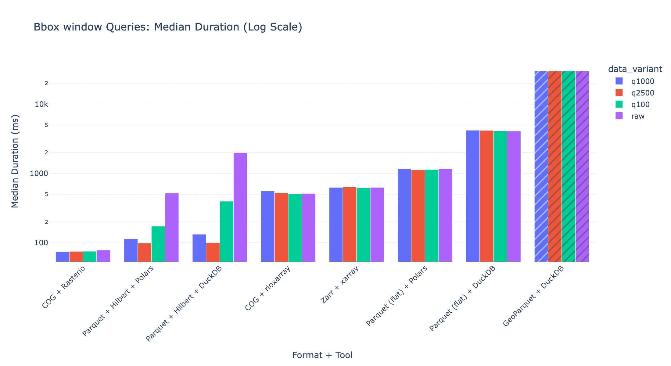
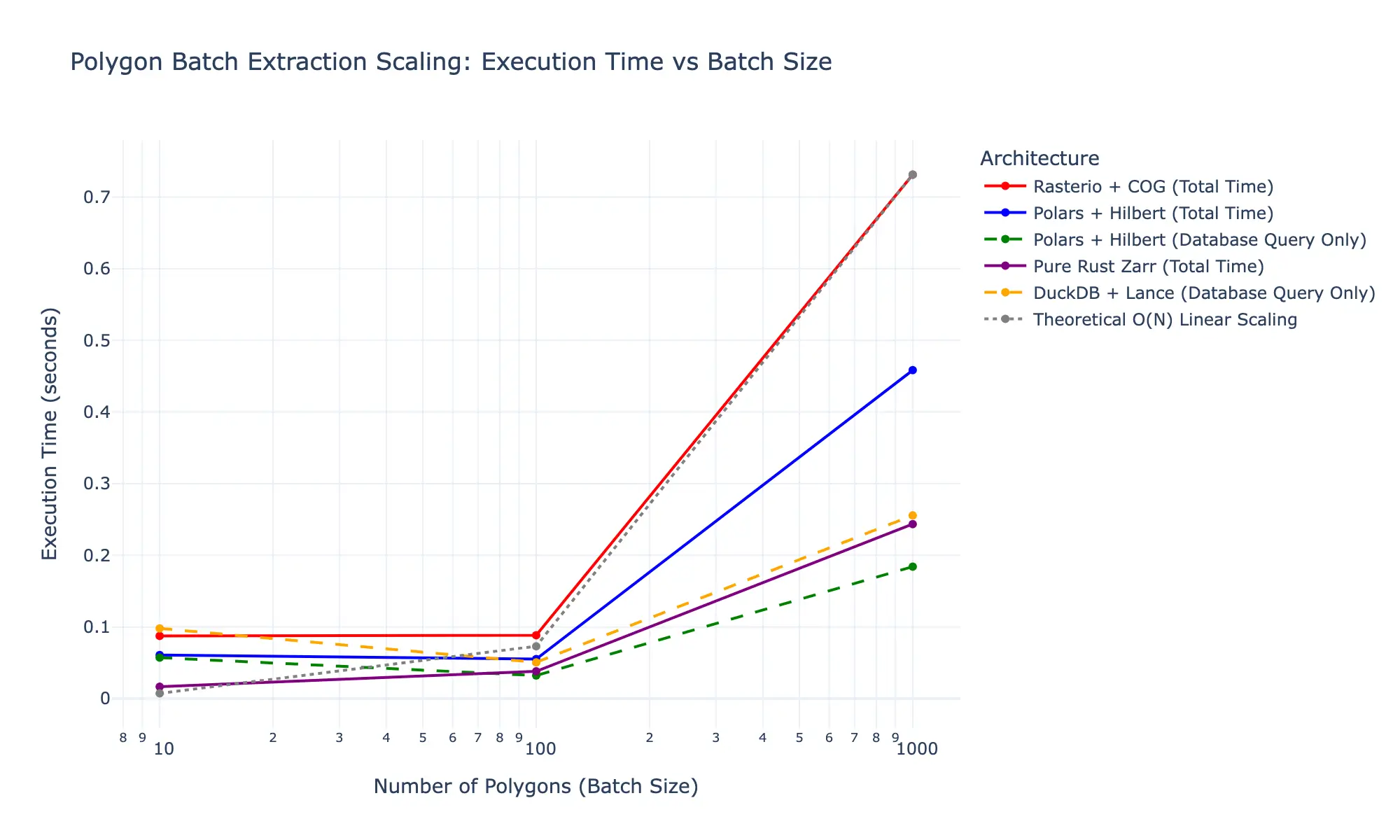
This is an O(N) sequential operation over geometries. At 1,000 polygons it takes 0.73 seconds locally. In production, querying global tiled COGs over cloud object storage inflates that to minutes, because every polygon triggers sequential HTTP requests, each carrying a ~50ms Time-To-First-Byte (TTFB) penalty that bandwidth alone cannot solve. For a platform designed to make physical climate risk as actionable as credit risk, that latency profile is a non-starter.
Six Architectures, One Test: What We Benchmarked
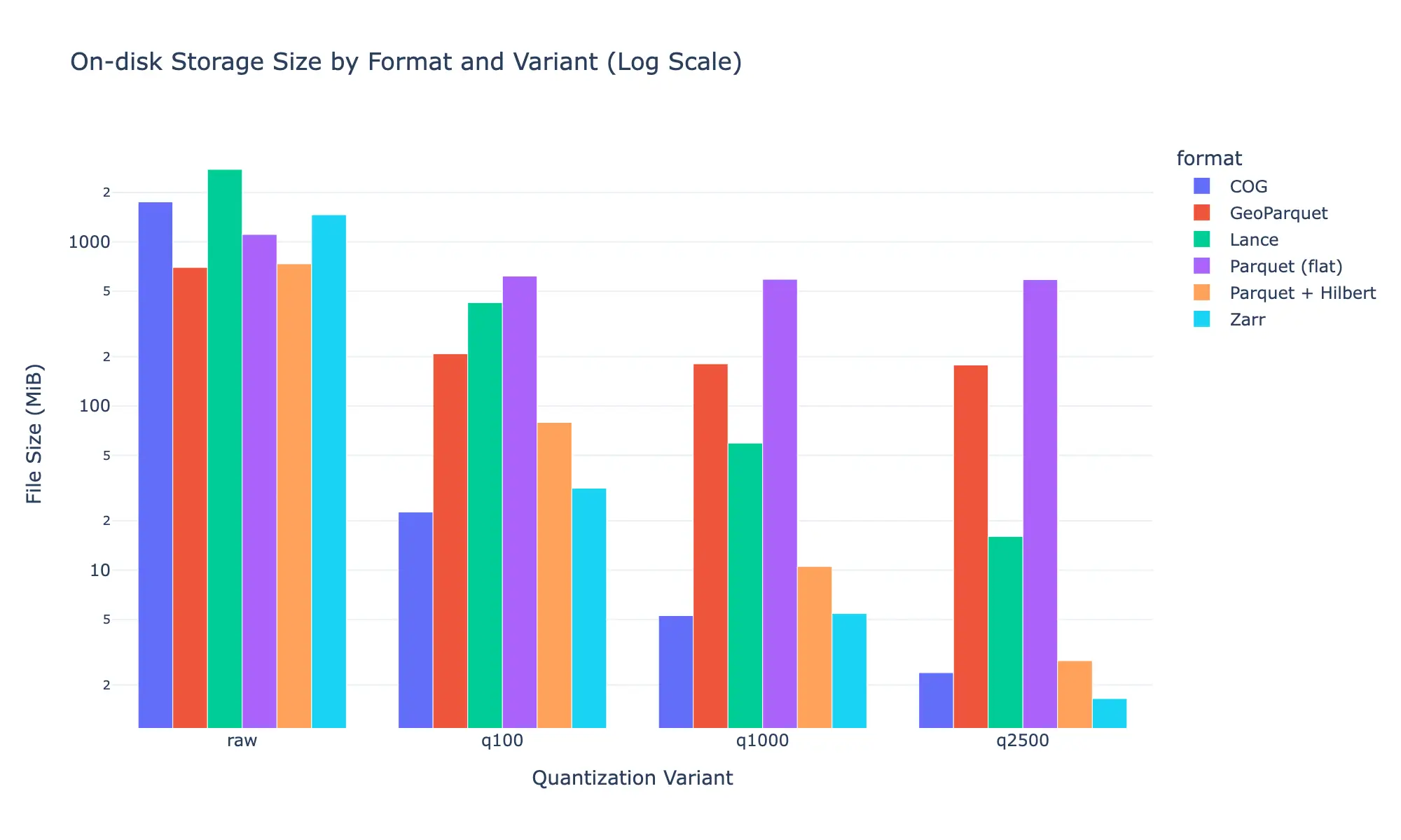
To find an architecture capable of meeting those constraints, we evaluated six distinct combinations of data formats and query engines against a controlled proxy dataset: a 6°×6° Copernicus Digital Elevation Model (DEM) at 30-metre resolution covering the Swiss Alps (1.7 GB, ~466 million pixels) quantised to simulate the categorical profile of real hazard data.
| # | Architecture | Approach |
|---|---|---|
| 01 |
Rasterio + COG
|
The industry standard. Sequential raster masking via Python/C++ GDAL bindings. |
| 02 |
Xarray + Zarr
|
Lazy-loaded N-dimensional arrays queried sequentially via Python. |
| 03 |
DuckDB + Parquet
|
Vectorised Hash Joins over 1D columnar data using an analytical SQL engine. |
| 04 |
Polars + Parquet
|
The same Hash Join approach via a high-performance Rust DataFrame library. |
| 05 |
Pure Rust Zarr (zarrs + geo-rasterize)
|
A custom backend bypassing Python entirely, querying Zarr chunks natively with asynchronous HTTP Range requests. |
| 06 |
DuckDB + Lance
|
Querying a format optimised for AI model data shuffling, using both SQL joins and its native Scanner. |
The Tabular Detour: Why Parquet Hash Joins Don't Work for Hazard Data
One alternative to raster masking is treating spatial data as tabular data. By flattening the pixel grid into a columnar Parquet file, you can use DuckDB or Polars to execute vectorised Hash Joins, in effect asking the database to find all rows whose spatial index falls inside the polygon.
To make this work without an explicit coordinate column for every pixel (the “Coordinate Tax”, which bloats a flat Parquet file for our proxy dataset to 1.1 GB), we mapped the global grid onto a Native 2D Hilbert Curve: a 1D integer that encodes each pixel’s position while preserving geographic locality.
The area-weighting flaw: why Quadtree compaction breaks EAL accuracy
For spatially uniform hazard data, this can be further compressed using Quadtree Compaction: recursively merging identical adjacent pixels into parent cells. Applied to a coarsely quantised dataset, this reduces storage from 1.1 GB to 2.8 MB.

However, this compaction introduces a critical flaw for production analytics: the area-weighting problem. In a compacted Quadtree, one row may represent a single pixel; another may represent 1,024 pixels. A simple AVG(hazard_value) query treats both equally, producing incorrect Expected Annual Loss calculations at polygon boundaries. That flaw is disqualifying when the outputs feed into credit risk frameworks and regulatory disclosures.
The Parquet approach also suffers from a structural I/O problem we call the Zone Map Trap. A 2D polygon, once flattened to 1D Hilbert indices, fragments across hundreds of non-contiguous row groups on disk. To find the 23 KB of data actually needed for a single polygon, DuckDB was forced to download and decompress 689 MB of irrelevant rows. This read amplification, not CPU performance, is the bottleneck in production.

Fixing this requires adding explicit X/Y coordinate columns back into the file (so the database can use 2D Zone Maps to prune irrelevant row groups before the join). That works, but it bloats the file from 319 MB to 528 MB. You pay the Coordinate Tax to fix the I/O problem you introduced by removing it.
The Architecture That Works: Native Rust + Zarr for Synchronous Climate Risk APIs
The winning approach bypasses both Python overhead and SQL complexity entirely.
We built a custom PyO3 extension in pure Rust using zarrs for direct, asynchronous byte-range fetching from Zarr chunks, geo-rasterize for high-performance polygon rasterisation, and rayon for multi-threaded parallel extraction.

Crucially, this approach yields mathematically correct AVG() aggregations, operating on raw pixels rather than compacted cells, with no area-weighting flaw. For EAL calculations that need to survive model risk management (MRM) review, that accuracy is non-negotiable.
If the data isn't fast enough, it doesn't get used. Real-time lending workflows don't accommodate minute-long API responses. When a loan origination team needs a climate risk assessment while a customer is waiting, the platform either responds within seconds or it gets bypassed entirely. The same applies to pre-origination screening across large collateral portfolios. Batch queries that take hours create operational bottlenecks that force manual workarounds, not better decisions.
Why Cloud I/O Is the Real Problem and Why Rust + Zarr is the Solution
The local benchmark results, a 0.49-second gap between Rasterio and Zarr for 1,000 polygons, might seem like an engineering footnote rather than an architectural imperative. It isn't.
Local benchmarks run on NVMe storage. In production, global hazard data lives in cloud object storage. Fetching data over S3 introduces a hard latency floor: every HTTP request carries approximately 50ms of Time-To-First-Byte (TTFB) latency. This is not a bandwidth problem. It is an inherent property of establishing TCP connections to remote object stores. No amount of network throughput eliminates it.
Standard GIS tools querying COGs must download complex TIFF header metadata before fetching any data tiles. Across 1,000 polygons and multiple hazard layers, each requiring separate header fetches and tile reads, those 50ms penalties compound until extraction times inflate from seconds to minutes.
The Rust + Zarr architecture is effectively immune to this penalty, for two reasons:
01. Metadata is trivial. Zarr's .zarray JSON metadata is approximately 1 KB regardless of how large the dataset grows. There is no per-layer IFD explosion, no TIFF header to download per spatial tile. The backend reads a single metadata file and uses simple arithmetic to calculate exactly which byte-ranges are needed for all 1,000 polygons and across all layers upfront.
02. Requests are concurrent. The Rust HTTP client fires all required byte-range requests in parallel, using connection pooling to manage socket limits efficiently. Modern object stores (AWS S3 handles over 5,500 GET requests per second per prefix) are designed for this pattern. The 50ms TTFB penalty is paid effectively once per batch, not once per polygon.
Scaling to 240 Terabytes: Why COG Fails at 700 Layers
With more than 700 distinct hazard layers per spatial pixel, the limits of traditional raster architectures become catastrophic rather than merely inconvenient.
Storing 700 layers as separate COG files would require downloading 700 separate IFD headers per query. At 50ms TTFB each, sequential header fetches alone would cost 35 seconds of pure network latency before a single pixel of data is touched.
Combining 700 bands into a single multi-band COG triggers a different problem: metadata explosion. A global 30m dataset chunked into 512×512 tiles generates ~3.38 million spatial tiles per band. Across 700 bands with band-interleaved storage, tracking tile offsets and byte counts requires a header that swells to ~37.8 gigabytes, which the client must download just to locate its data.
Pixel-interleaved COG compresses the header (down to ~54 MB) but introduces catastrophic bandwidth overfetching: querying a single hazard layer forces the client to download and discard the other 699 layers for every chunk it touches.
Zarr sidesteps all of this. Its metadata remains constant at ~1 KB regardless of dimensionality. Its N-dimensional chunking, structured as [layer, y, x], allows the Rust backend to calculate the precise byte-offset for a single layer within a single spatial chunk and read only those bytes, leaving everything else untouched.
Regulated institutions need trusted the data. A climate risk score without a traceable methodology creates a problem, not a solution. Risk and model validation teams at banks and insurers need to understand where numbers come from, how uncertainty is handled, and whether the approach will survive regulatory scrutiny. We ensure every Spectra climate risk score is backed by a transparent, traceable methodology.
Zarr v3 Sharding: Solving the File Count Problem
One remaining challenge: Zarr v2 stores every chunk as an individual file. A global 30m dataset with 700 layers chunked into 512×512 grids generates billions of files, enough to exhaust inode limits on caching layers, slow data transfer, and inflate PUT/LIST costs.
The solution is Zarr v3 Sharding: grouping thousands of chunks into larger Shard files (~500 MB), with a byte-offset index appended to each shard. When querying:
-
01Read master metadata to locate the relevant Shard file.
-
02Fetch the trailing byte-offset index via an HTTP Range request.
-
03Parse the index to locate the specific inner chunk.
-
04Fetch the required bytes via a second HTTP Range request.
This introduces a "double-fetch" penalty, but only once per shard, and only when that shard's index is not yet cached. In practice, query patterns for asset-level analytics tend to be geographically clustered: a bank screens collateral within a lending region, a fund manager assesses assets within a portfolio. Shard indices for those areas stay hot in memory, and subsequent queries within the same geography resolve with a single Range request.
Architectural Summary: Comparing Approaches to Climate Risk Data at Scale
| Architecture | Storage | Latency (1K polygons) | Scaling | Correct AVG() | Cloud I/O Penalty |
|---|---|---|---|---|---|
| COG + Rasterio | 2.4 MB | 0.73s | Linear O(N) | Yes | High (sequential headers) |
| Parquet (Compacted) + DuckDB | 2.8 MB | 0.18s | Sub-linear | No (area-weighting flaw) | Low |
| Parquet (Uncompacted X/Y) + DuckDB | 528 MB | ~0.10s | Sub-linear | Yes | Low (2D Zone Maps) |
| Lance + Scanner | 4,700 MB | 1.02s | Sub-linear | Yes | Low |
| Zarr v3 + Pure Rust | 1.7 MB | 0.24s | Flat | Yes | None (concurrent requests) |
What the Benchmarks Tell Us and What It Means for Investment-Grade Climate Analytics
The results point clearly in one direction. A pure-Rust backend querying sharded N-dimensional Zarr arrays is the only architecture that simultaneously satisfies all four requirements for production-grade physical climate risk analytics: competitive storage size, mathematically correct aggregations, synchronous API performance, and immunity to cloud I/O penalties at multi-hundred-terabyte scale.
The trade-off is real. Introducing a compiled Rust extension into a Python data engineering stack adds pipeline complexity: cross-language debugging, CI/CD compilation steps, a steeper on-boarding curve for engineers coming from a pure Python background. But because the underlying mathematics of geographic chunk intersection and binary rasterisation are effectively immutable, this is a stable, well-bounded cost. The Rust layer, once written, does not need to change as the dataset grows.
The broader point matters for anyone building in this space. Physical climate risk data is not like most financial data. It is inherently spatial, multi-dimensional, and global. The tools that work for time-series data, for tabular credit data and for columnar market data, break in predictable, well-understood ways when you apply them here. The engineering decisions required to deliver EAL calculations at asset level, across 11 hazards, at synchronous API speeds, are non-trivial. Getting them right is part of what separates a platform that can support real investment decisions from one that can only support static reports.
Physical climate risk only gets priced into investment decisions when the data is both accurate and fast enough to be useful. This benchmark is our evidence that the right architecture for that exists.
Why the data engineering behind climate risk analytics matters.
Why does COG fail for large-batch asset screening?
Cloud Optimised GeoTIFF was designed for single-asset or small-batch queries over the web. It works well in that context. It breaks down when you need to screen hundreds or thousands of assets simultaneously, which is the standard use case in portfolio due diligence and pre-origination collateral checks.
The problem is sequential I/O. Every polygon triggers a separate chain of HTTP requests: fetch the TIFF header metadata, locate the relevant spatial tiles, decompress and mask them. Each request carries a hard latency floor of roughly 50ms. Not because of bandwidth, but because of the cost of establishing TCP connections to cloud object storage. That penalty compounds across a large batch until extraction times stretch from seconds into minutes. For a platform that needs to return results within standard API timeouts, that latency profile isn't workable. At multi-hundred-terabyte scale, across 700+ distinct hazard layers, the problem becomes structural rather than marginal.
What is Average Annual Loss (AAL) and how is it calculated?
Average Annual Loss is the expected financial loss from a given climate hazard in any given year, expressed as a monetary figure and averaged across all possible loss events weighted by their probability of occurrence. It captures both frequent, lower-severity events and rare, high-severity ones, giving a single metric that reflects the full distribution of risk rather than any single scenario.
In practice, AAL is calculated by integrating hazard probability and loss severity across multiple return periods: the 1-in-10-year event, the 1-in-100-year event, and so on, then summing the probability-weighted outcomes. Getting that calculation right at asset level, across 11 hazards and multiple emission scenarios, requires the underlying data query to return mathematically precise pixel-level values. Spatial data compression techniques that average or merge adjacent pixels introduce systematic errors that distort the AAL figure, which is why the architecture described in this post matters. Spectra delivers AAL at asset and portfolio level, with methodology documentation designed to withstand model risk management review.
How does Zarr compare to GeoTIFF for climate risk analytics?
Both formats store gridded spatial data, but they're built for different access patterns. GeoTIFF, and its cloud variant COG, organises data in 2D spatial tiles and uses a metadata index to locate them. That structure works for a limited number of layers and sequential queries. It doesn't scale to the dimensionality that credible physical climate risk modelling demands: 700+ layers per spatial pixel, queried in parallel for thousands of assets.
Zarr stores data as an N-dimensional array with a simple JSON metadata file of roughly 1 KB, constant regardless of how many layers the dataset contains. Its chunk structure maps directly onto the data's physical dimensions, so a query for a single hazard layer across a specific geography touches only the bytes it needs and nothing else. That precision matters in cloud environments where every unnecessary read is a latency cost. The Zarr approach also allows all required byte-ranges, across all 1,000 polygons and all hazard layers, to be fetched concurrently rather than sequentially. That's the difference between seconds and minutes at production scale.
What does 30-metre resolution mean for physical climate risk?
At 30-metre resolution, each data pixel covers a ground area of roughly 900 square metres, close to plot level and well within the footprint of most individual assets. This matters because climate hazard exposure varies substantially at short distances. A building on one side of a road may sit inside a flood plain; the building opposite may not. Postcode-level or regional data averages that difference away. At 30-metre resolution, it's preserved.
For financial institutions, the implication is direct: asset-level risk scores computed from coarser data will misstate exposure for a meaningful fraction of any portfolio. That error compounds at scale. A lending book with 50,000 properties assessed at regional resolution carries systematic inaccuracy in its collateral risk estimates, which creates problems both for internal credit risk frameworks and for regulatory stress tests that require granular, defensible inputs. Thirty-metre resolution isn't a technical specification for its own sake. It's the minimum required to produce AAL figures that hold up at the asset level.
How does this architecture support model risk management (MRM) review?
MRM teams within financial institutions are tasked with validating vendor models before they can be used in credit risk, stress testing, or capital adequacy frameworks. The most common reason vendor climate risk models fail MRM review is opacity: scores that can't be traced back to their inputs, or methodologies that can't be independently reproduced.
The architecture described in this post is designed with that constraint in mind. Every step, from the raw CMIP6 climate projections through hazard modelling to the final pixel-level AAL calculation, produces outputs that can be interrogated and verified. The Zarr data structure stores hazard values as raw pixels rather than compressed or merged cells, so the aggregation logic is transparent and mathematically verifiable. There are no intermediate approximations that distort the result. Spectra's methodology documentation covers the full chain from climate inputs to financial outputs, giving MRM teams the evidence trail they need to validate the model within their internal governance frameworks.
Our Latest Articles & News
A selection of some of our latest articles covering industry, policy and climate science - written by us.


